Understanding Neural Networks
Neural networks generate a lot of interest. However, it’s not always clear to people outside of the machine learning community the problems they’re suited for, what they are, or how they’re built. We’ll address these topics in this blog post, aiming to make neural networks accessible to all readers. For those with programing experience, I’ve appended a Jupyter Notebook at the end which you can follow to build your own neural network.
Most commercially successful applications of neural networks are in the area of supervised learning. In supervised
learning, we are trying to build a model that maps inputs to outputs. Some examples include:
| Input | Output |
|---|---|
| Is this spam or not? | |
| User feedback | How positive is the feedback? |
| Internet ad | Will a user click on this ad? |
| Speech Audio File | The speech as text |
| Satellite image of the ocean | Outlines of all the ships |
| Picture of a material | Is there a defect? |
We can represent these models as function that takes an input and produces an output:
y = F(x)
where x is the input, y is the output, and F() is our model. Neural networks are a particularly effective way to build a model (i.e. F() ) for many classes of problems.
Let’s briefly consider a traditional approach for building many models. We can derive models describing many phenomena by applying our understanding of calculus to specific domain knowledge. In physics, this would include Newton’s Laws of Motion, or conservation laws stating that mass, energy, and momentum are conserved in a closed system. This approach let’s us successfully build a variety of important models, such as the ideal rocket equations which tell us tell us how much fuel a rocket needs to reach space, or the Boussinesq equations which let us model waves along the coast.
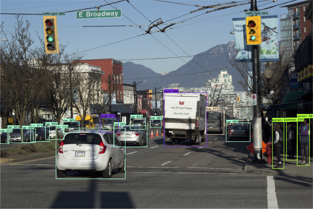
What about problems for which we don’t have intuition into the fundamental dynamics? Say you are building an autonomous vehicle, and want to recognize other cars on the road using a video stream from your dashboard camera. Despite the fact that we’re all quite good at recognizing cars, we haven’t been able to formulate physical principles describing what a car looks like. We can’t point to a combination of wheels, doors, and windows which make up a car. Neural networks provide us a technique which we can use to solve these types of problems effectively.
Neural networks work by learning the mapping from input to output directly from data. The process of having the neural network learn this mapping is known as training. Training requires a dataset of training examples, which are pairs of inputs and the corresponding outputs (x and y). For training to be effective, we need a large dataset, typically tens of thousands to tens of millions of training examples.
During training, we are optimizing the weights (or parameters) of the neural network. For each training example, we run the model on the input, and compare the model output to the target output using a loss function. Using an algorithm called backpropogation (or backprop for short), we update all the weights in the network so that the model output will be closer to the target output. The weights are updated proportionally to how much they contribute to any mismatch. We continue cycling through our training set, iteratively updating the model, until performance no longer increases.
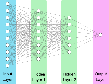
Let’s look at a visualization of a straightforward neural network. On the left hand side we have the input layer. This is our data, such as the pixels of an image, or how many times certain words appear in an email. Next we have two hidden layers. Hidden layers is a term we refer to the layers between the input and the output layers. Finally, we have the output layer. As the input passes through each layer of the neural network, it undergoes a series of computations. Each ‘unit’ (or ‘neuron’) in the hidden layers and the output layer contain a set of weights to be optimized, which control these calculations.
Designing a neural network requires selecting hyper-parameters controlling both the architecture of the network and the training process. We use the term hyperparameters, since the term parameters is an alternative to weights. Hyperparameters related to the architecture include the number of layers, the width of each layer (i.e. number of units), as well the choice of something called the activation function in the units. The training is particularly influenced by the choice of optimization algorithm, the learning rate used by the algorithm, and whether a technique called regularization is implemented.
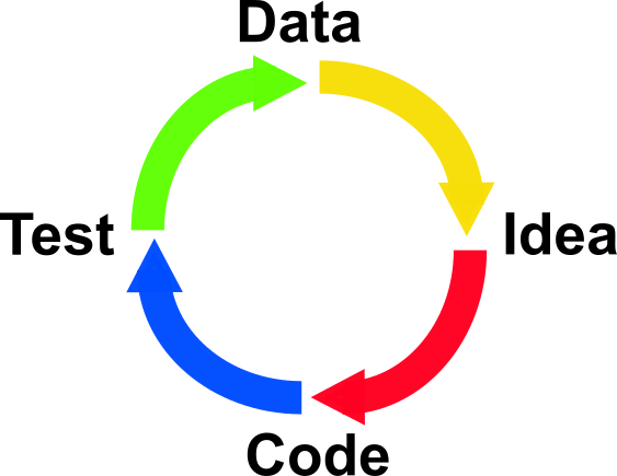
Unfortunately, there is no way to know beforehand what is the best architecture for your problem, or what the best parameters for training that architecture would be. Practitioners are guided by a combination of experience, intuition, and best practices from the community. As the field is moving rapidly, this requires continuously staying up to date. Often the best way to start on a problem is to look at the machine learning literature to see if someone has solved a problem similar to yours, and take their solution as a starting point. Getting a solution to your particular problem will usually require several iterations of looking at the data, realizing ideas, modifying the model code, and testing.
A key question of any neural network is how well is it able to perform on data it hasn’t seen before. Therefore, before training a neural network, a small portion of the data is set aside in what is commonly referred to as the test set. Following training a neural network, we compare the performance of the neural network on the training set and the test set. One possible scenario is that the model doesn’t perform well even on the data its trained on. In case, we say the model has high bias. When the model doesn’t fit the data it has seen well, the hyperparameters should be reevaluated. Another outcome is that the model performs well on the training set, but not very well on the test set. In this situation, we say the model has high variance – that the neural network has been overfit to the training data. Equivalently, the network hasn’t learnt features of the data that generalize well, and perhaps has memorized features specific to the training set. To address high variance, we typically employ a technique called regularization. When feasible, acquiring additional data is also beneficial.
An important detail is that the data you train your neural network has to be similar to the data you apply your neural network to. Statistically, you want your training and test data to come from the same distribution. Intuitively, this means if you train your autonomous vehicle to drive exclusively in sunny weather, you can’t expect it to stay on the road during a snowfall. In practice, this means if you develop a neural network to predict customer behaviour, you’ll need to update your model periodically as your important factors such as your products, customers, and competition evolve.
These are the broad concepts key to understanding how to apply neural networks, and communicate with those who regularly work with them. After reading this, you should be able to confidently navigate a conversation on applying neural networks.
To summarize the key points about neural networks:
- They are an effective way to build a model mapping from input to output directly from a training dataset.
- Neural networks have many hyperparameters, and designing a good network is an iterative process.
- Your training and test data should come from the same distribution.
Finally, a lot of software developers I speak to are keen to know implementation details of neural networks. The following Jupyter Notebook details has been designed with you in mind, implementing a neural network to recognize handwritten digits with 98% accuracy. We’ll assume you have python environment setup with PyTorch. If you don’t, Anaconda is the recommended package manager and pretty simple to get started with.
You can download the jupyter notebook to run on your own machine here, as
well as follow along with the precomputed version below.
MNIST Jupyter Notebook
Let’s begin by importing the necessary modules. We’ll use matplotlib for plotting, pytorch as our machine learning framework, the time module for tracking the length of calculations, and numpy for array manipulations.
import matplotlib.pyplot as plt
import time
import numpy as np

import torch
import torchvision
import torch.nn as nn
import torch.nn.functional as F
from torch.utils.data import DataLoader
Next, let’s acquire and load the MNIST dataset. Since this is a common dataset, the torchvision module has a class that
simplifies this procedure. The following lines of code downloads the MNIST dataset, which is conveniently divided into
a test and training set. The dataset is stored in the directory assigned to data_dir.
The MNIST dataset provides images in a Python Image Library (PIL) format. We’ll have torch automatically apply a transform to these images to convert them to tensors.
data_dir = './data'
pil2tnsr = torchvision.transforms.ToTensor()

train = torchvision.datasets.MNIST(data_dir, train=True, download=True, transform=pil2tnsr)
test = torchvision.datasets.MNIST(data_dir, train=False, download=True, transform=pil2tnsr)

print(f'Number of images in training set: {len(train)}')
print(f'Number of images in test set: {len(test)}')
Number of images in training set: 60000 Number of images in test set: 10000
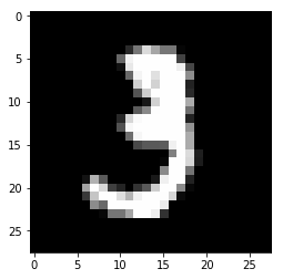
Now that we have the MNIST dataset, let’s see what images look like. The variable index specifies an image number
in our training set. Change it to explore other entries in the dataset.
index = 10
img, label = train[index]

tensr2pil = torchvision.transforms.ToPILImage()
img_pil = tensr2pil(img)

plt.figure()
plt.imshow(img_pil)

print(f'Image label: {label}')
print(f'Image size: {img_pil.size}')
Image label: 3 Image size: (28, 28)
PyTorch provides useful tools to simplify loading and processing our data. Since we used torchvision to get the MNIST
dataset, train and test are already objects which PyTorch recognizes as datasets. We can pass them to
DataLoader, which simplifies iterating through the dataset. Setting batch_size to 8 means we’ll iterate through 8
images/labels at a time, and setting shuffle to True means that data is shuffled after we have iterated through the
entire dataset.
train_loader = DataLoader(train, batch_size=8, shuffle=True)
test_loader = DataLoader(test, batch_size=8, shuffle=True)
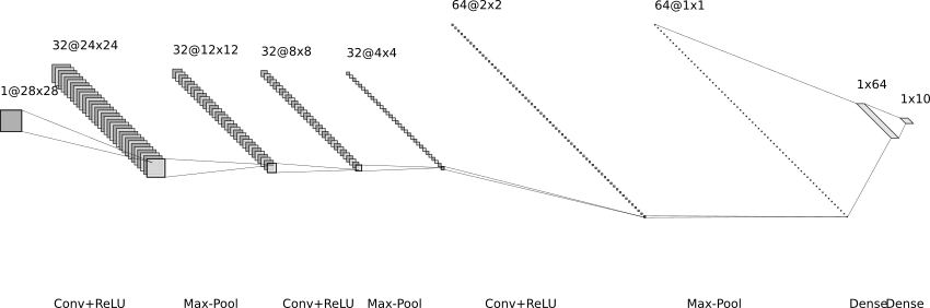
Here we define our neural network. We use a fairly simple convolutional neural network architecture. The first part of the network has three repetitions of a convolutional layer with a ReLU activation followed by a maxpooling layer. Afterwards, there are two fully connected layers with a ReLU activation between them.
class Net(nn.Module):

def __init__(self):
super(Net, self).__init__()

self.conv1 = nn.Conv2d(1, 32, 5)
self.conv2 = nn.Conv2d(32, 32, 5)
self.conv3 = nn.Conv2d(32, 64, 3)
self.dense1 = nn.Linear(64, 64)
self.dense2 = nn.Linear(64, 10)
self.maxpool1 = nn.MaxPool2d((2, 2), stride=(2,2))


def forward(self, x):
#Conv/pool: (Batch size, 1, 28,28 ) -> (Batch size, 32, 24, 24) -> (Batch size, 32, 12, 12)
x = F.relu(self.conv1(x))
x = self.maxpool1(x)

#Conv/pool: (Batch size, 32, 12, 12) -> (Batch size, 32, 8, 8) -> (Batch size, 32, 4, 4)
x = F.relu(self.conv2(x))
x = self.maxpool1(x)

#Conv/pool: (Batch size, 32, 4, 4) -> (Batch size, 64, 2, 2) -> (Batch size, 64, 1, 1)
x = F.relu(self.conv3(x))
x = self.maxpool1(x)

#Flatten: (Batch size, 64, 1, 1) -> (Batch size, 64*1*1)
x = x.view(-1, 64)

#Dense Layer 1: (Batch size, 64) -> (Batch size, 64)
x = F.relu(self.dense1(x))

#Dense Layer 2: (Batch size, 64) -> (Batch size, 10)
x = self.dense2(x)

return x
Let’s instantiate our neural network. We’ll also need to choose a loss function. Here we’ve selected Cross Entropy Loss, which is appropriate when you want your neural network to assign your input to one of several classes. We’ve selected the Adam optimization algorithm to optimize our network weights such that they minimize our loss function.
model = Net()

loss_function = nn.CrossEntropyLoss()
optimizer = torch.optim.Adam(model.parameters(), lr=1e-3)
We have everything we need to go. This code iterates through our data, comparing the model prediction with the labels,
and updating our weights to improve our neural networks ability. The num_epochs parameters determine how many time
we cycle through our dataset.
torch.manual_seed(1)

num_epochs = 2

#Initalize counters
running_loss = 0.0
correct = 0.0
total = 0.0

for epoch in range(num_epochs):
print(f'Epoch: {epoch+1}/{num_epochs}')
t_start = time.time()

#Iterate through mini-batches
for i, data in enumerate(train_loader,0):

#Optimize the neural network
inputs, labels = data
y_pred = model(inputs)
loss = loss_function(y_pred, labels)
optimizer.zero_grad()
loss.backward()
optimizer.step()

#Track the accuracy of its predictions
_, predicted = torch.max(y_pred.data, 1)
total += labels.size(0)
correct += (predicted == labels).sum().item()

#Track the loss function, and output it regularly
running_loss += loss.item()
if i % 2000 == 1999:
print(f'Loss: {running_loss/2000}')
running_loss = 0.0


print(f'Finished in {time.time() - t_start:.2f}s')
print(f'Accuracy on train set: {100*correct/total}')

running_loss = 0.0
correct = 0.0
total = 0.0
Epoch: 1/2 Loss: 0.30464214020967484 Loss: 0.1003953853920102 Loss: 0.0807381663620472 Finished in 107.92s Accuracy on train set: 95.54833333333333 Epoch: 2/2 Loss: 0.04743631257861853 Loss: 0.05301460570842027 Loss: 0.05167941872775555 Finished in 100.07s Accuracy on train set: 98.435
Great, our neural network is performing well. After 2 epochs of training, our neural network can correctly label images in the training set with 98.4% accuracy. How does it do on data it hasn’t seen before? Let’s check it’s performance on the test set.
correct = 0.0
total = 0.0
with torch.no_grad():
for data in test_loader:
inputs, labels = data
y_pred = model(inputs)
_, predicted = torch.max(y_pred.data, 1)
total += labels.size(0)
correct += (predicted == labels).sum().item()

print(f'Accuracy on test set: {100*correct/total}')
Accuracy on test set: 98.85
We see a slightly higher accuracy on the test set than on the training set. This means we haven’t overfitted the model, or in other words, in generalizes well.
Finally, let’s see our predictions.
dataiter = iter(test_loader)
images, labels = dataiter.next()

def imshow(img):
npimg = img.numpy()
plt.imshow(np.transpose(npimg, (1, 2, 0)))

imshow(torchvision.utils.make_grid(images))
plt.show()

print(labels)
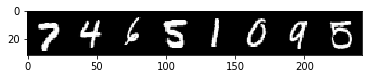
tensor([7, 4, 6, 5, 1, 0, 9, 5])
There you have it, a fully trained and functioning neural network capable of identifying handwritten digits with 98% accuracy. Similar networks have been deployed before to help read addresses on envelopes and writing on cheques.
Let’s summarize the ground we covered in this notebook:
- Loading Data
- Creating a neural network
- Selecting a loss function
- Optimizing your model
- Calculating the train and test set accuracy
- Making predictions with your model
The process used in this notebook is typical of machine learning projects. The code here is a good starting template for your own projects!